Optimizing Trajectories

2020-07-17

Something that came up recently is the optimization of trajectories. Imagine that you are given a very dense trajectory as a sequence of points. How can we simplify this trajectory, reducing the number of points while maintaining the original shape?

In the given trajectory, points could lie on the same line and therefore be redundant; two points are enough for the representation of a line segment. But the trajectory can also turn around, in which case more points are needed to properly describe the turn. The goal, then, is to remove those redundant points in the relatively straight segments of the trajectory while maintaining an appropriate number of points on the curves to maintain the original shape.

I would also like to come up with a simple solution that performs a decent job without getting into more complex maths. At this point, let me introduce a few assumptions:

The points are assumed to have a position only. If points have other properties like speed, acceleration, heading, etc, then the problem gets a bit more complicated, though the idea is fundamentally the same.
I will not be using splines or any advanced methods for simplicity.

The main idea behind this solution is to consider three consecutive points at a time, as shown below. Points are redundant when they lie on the same line. Points forming an angle are less redundant as the angle increases:

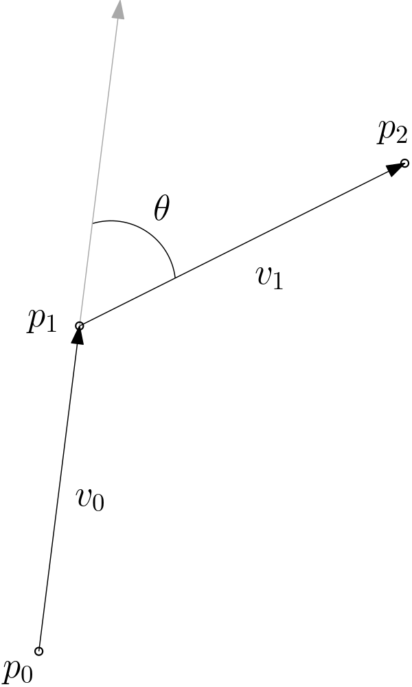
\(v_0\) is the normalized vector from \(p_0\) to \(p_1\), and \(v_1\) is the normalized vector from \(p_1\) to \(p_2\). If the three points lie on the same line, then the angle between the two is \(0\), which we can express with the dot product:

\[v_0 \cdot v_1 = \pm 1\]

The \(+1\) case is the one we want to optimize. \(-1\) occurs when \(v2\) is in the opposite direction of \(v1\), which represents a sudden turn of \(180°\). This case we do not want to optimize; the three points are required to represent that sudden turn. This observation of the dot product between the vectors formed by three consecutive points is the main idea behind the algorithm.

In practice, the three points are unlikely to lie exactly on the same line, so we can introduce an error threshold to determine whether the points are roughly on the same line. The larger the error, the more of the trajectory gets optimized away and less of the original shape is preserved.

The algorithm starts at the first point of the trajectory and considers the first three consecutive points. Then it asks the question: how much does the third point deviate from the line formed by the first two? If the angle is small, then we can remove the middle point without altering the trajectory too much. If it is big, then we should leave the middle point. The algorithm computes an error based on this angle, makes a decision based on it and the error threshold given as an input, and then moves on to the next three consecutive points starting at the second or third point, depending on the outcome of the decision. In other words, we do not consider points 1-3 in the original trajectory and then 4-6; we instead advance by one and look at points 2-4 or 3-5 depending on whether 2 was removed.

One thing to note is that if we only look at the local error for a given triplet of consecutive points, the algorithm is prone to eating away curves. This is because as we travel along a dense curve, the local error at every step could be below the threshold and the middle point discarded at every step. Here is an illustration:

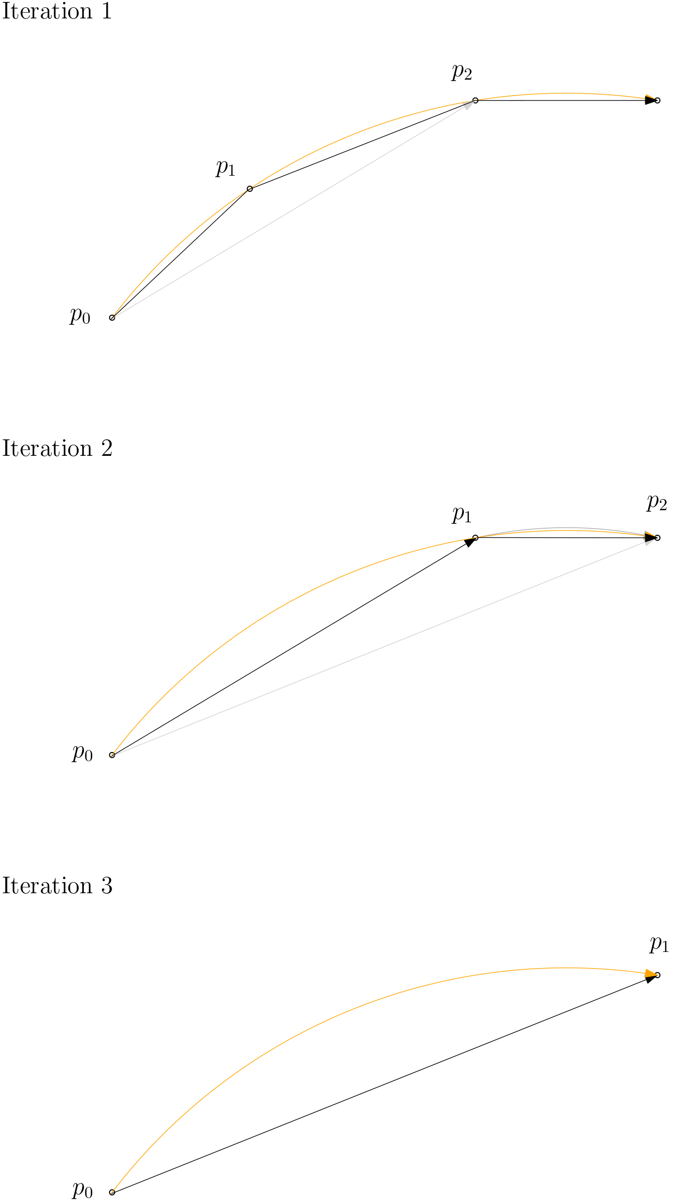
Instead, the algorithm must accumulate the error as it proceeds along the curve. The local errors may be small, but as they are accumulated, the sum grows larger and eventually beats the threshold. At that point, the algorithm decides not to optimize away the middle point, resets the error back to \(0\), and “starts again” from the next triplet.

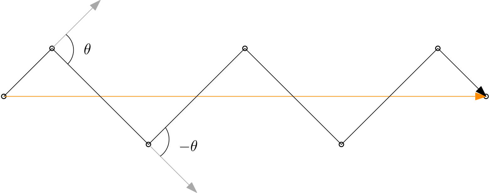
A final note and improvement is to make the error signed. We can make errors due to a left turn negative and errors due to a right turn positive (or vice versa, the distinction does not matter). In this way, when we accumulate the local errors, errors due to left turns cancel errors due to right turns. To see how this could be important, consider a trajectory that zig-zags its way from start to finish. If we work with positive errors only, then at some point the accumulated error beats the threshold and the algorithm “inserts” (decides not to optimize away) the middle point. This could make the algorithm leave many points along the way that are undesirable. Instead, by using signed errors, the “zig” cancels the “zag” and the algorithm outputs a straight line defined by the very first and last points of the trajectory.

And that is all. What follows is an implementation followed by some discussion. At the end of post, I also explore some further improvements we could make to the algorithm presented here.

/// Optimize the given trajectory in place.
/// `angle_threshold` must be in the range [0, pi/4].
fn optimize(angle_threshold: f64, trajectory: &mut Vec<Vec2>) {
  let th = 1.0 - f64::cos(angle_threshold);  // Positive number.
  debug_assert!(th >= 0.0);
  let mut error: f64 = 0.0;
  let mut i = 0;  // First point.
  let mut j = 1;  // Second/middle point.
  let mut k = 1;  // Index into the next element of the result vector.
  while i < trajectory.len() && j < trajectory.len() {
    //println!("i: {}, j: {}, k: {}", i, j, k);
    if j + 1 == trajectory.len() {  // Reached the end, insert last point.
      trajectory[k] = trajectory[j];
      k += 1;
      break;
    }
    let v0 = Vec2::normalize(trajectory[j] - trajectory[i]);
    let v1 = Vec2::normalize(trajectory[j+1] - trajectory[j]);
    let tg = Vec2::tangent(v0);
    let sgn = if Vec2::dot(v1,tg) >= 0.0 { 1.0 } else { -1.0 };
    error += (1.0 - Vec2::dot(v0,v1)) * sgn;
    //println!("error: {}, th: {}", error, th);
    if f64::abs(error) > th {  // Insert the middle point.
      trajectory[k] = trajectory[j];
      i = j;
      j += 1;
      k += 1;
      error = 0.0;
    } else {  // Skip the middle point.
      j += 1
    }
  }
  trajectory.resize(k, Default::default());
}

Full source code

There are three things to note in this implementation. The first is that the implementation mutates the input trajectory in place as opposed to allocating space for a new one. An implementation that creates a second trajectory might be easier to implement and read, but it also imposes an extra memory allocation.

The second thing to note is that instead of working with the angular error directly, we work with its cosine instead. The reason is that if we compared angles, we would have to transform the dot product into an angle by computing acos(), and this can be expensive since it happens at every iteration. Instead, we keep the dot product as is and compare it against the cosine of the input angular error.

Finally, you can comment out the println() statements to see the algorithm in action.

Improvements

The proposed algorithm works under the assumptions stated at the very beginning of this post. Let’s briefly discuss further improvements we could make on the algorithm so far.

Additional point properties

Points in the trajectory can have additional properties, like a speed that determines how fast an object travels between the current point and the next one. The algorithm presented here takes care of the geometrical aspect of the trajectory only and ignores all these other properties. In the presence of speed, for example, the algorithm would yield incorrect results. Imagine a straight line with multiple trajectories but differing speeds at every point; if we eliminate the middle points, we could be changing the speed at which the object travels from the first point to the last one.

The good news is that handling speed and other properties is no different than what we have done for the geometry of the curve: calculate the error we would induce by removing the middle point, and proceed until the accumulated error beats a threshold. This makes the implementation more terse, but the fundamental idea is the same. It can be terse especially because now the algorithm would take two threshold parameters instead of one: the angular error threshold and a new speed error threshold.

Handling noise

The algorithm presented here does not handle noise. It asumes that the input trajectory is in a good shape, just partially redundant. If the points in the input trajectory are the result of sampling an object’s position over time and they are known to be off the real trajectory, then the algorithm presented here is not ideal to reconstruct the original trajectory. A more general and robust curve-fitting algorithm is needed.

Splines

Like we mentioned earlier, a more optimized trajectory can be obtained by using splines.